

202
P. Wang et al. / Coastal Engineering 46 (2002) 175211
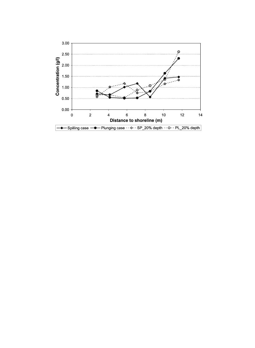
Fig. 22. Time- and depth-averaged sediment concentration, compared with measurements at an elevation of 20% water depth from bed.
Limited by the paucity of field and laboratory data
urements were taken, was significantly lower than the
and the incomplete understanding of surf-zone pro-
depth-averaged concentration.
cesses, present models are not yet capable of precisely
predicting instantaneous surf zone velocities and sedi-
4.5. Calculating sediment flux from current velocities
ment concentrations. Temporally and spatially aver-
and sediment concentrations
aged values are used in most modeling efforts. As
discussed earlier, by partitioning the surf-zone current
Eq. (1) yields a point value of sediment flux in
and sediment concentration into mean, high-frequency
space and time. It is necessary to integrate the point
and low-frequency components (Eqs. (3) and (4)),
values over space and time to obtain a sediment
calculation of time-averaged sediment transport (still
transport rate for practical use in coastal engineering
in a single point) can be obtained from Eq. (5).
and science. Knowledge of temporal and spatial dis-
Application of Eq. (5) in sediment transport modeling
tribution patterns is critical in performing the integra-
is difficult due to our limited abilities in predicting
tion and selecting proper temporal and spatial scales.
current and sediment concentration at a temporal scale
As discussed in the previous sections, longshore and
comparable to the frequencies of gravity and infra-
cross-shore currents and sediment concentrations vary
gravity waves. In the following, possibilities and
rapidly and differently in time and space. This makes
uncertainties of further simplification of Eq. (5) are
the integration, potentially, very complicated over a
examined by considering only the time-invariant
realistic domain.
terms.
Sediment flux is typically calculated via Eq. (1)
Neglecting the time-varying contributions, i.e., the
using velocity and concentration data obtained from
last two terms on the right-hand side of Eq. (5), can be
flow and turbidity sensors, respectively. Due to the
justified under two conditions. Condition one is sat-
high costs of sensors and field operations, temporal
isfied when either the temporal variation of one or both
and spatial coverage is often limited. Miller (1998,
of the two parameters, i.e., the u_high and u_low or c_high
1999) obtained a unique set of storm data in the surf
zone with simultaneous measurements of velocities
and c_low, over the averaging period are sufficiently
and sediment concentrations at Duck, NC. The 500-
small compared to the average values. Condition two is
m-long concrete pier and a 70-ton crane, allowed
satisfied when u and c are independent random varia-
bles with a zero mean and the time averages of u_high
measurement to be made under breaking waves of
c_high and u_low c_low, are negligible.
nearly 4 m high.

 Previous Page
