

ERDC/CHL CHETN-VII-5
December 2003
as a transport rate. However, when posing the method as a solution of the Exner equation, it becomes
clear that the change of volume, and thus the change or gradient of transport, is being measured, and
not the transport. So the ordinates of the graphic results presented in Abraham (2002), should be
stated as ∆q (q2 - q1), and not as q, where q is the transport of bed material in the sand waves in mass
per time per unit width of channel. That being said, it is interesting to note that the ∆q approaches q
as the time-step, or interval between successive bathymetric plots, gets small. Further analysis is
necessary to determine if this is always the case, and if so, to understand why it is so. Preliminary
results are encouraging, and after applying the method to several real river examples it is becoming
clear that the method can already be used in a relative sense. Because of the repeatability of the
measurements and consistency of the method, relative differences between two or more
measurement events appear to be able to quantify real changes. However, it is acknowledged that
more measurements, experience and statistical analysis must be made in order to prove this
statement in a more rigorous sense.
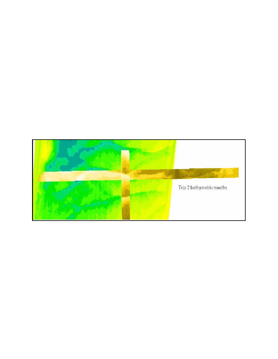
Figure 2 shows the portion of the study area where detailed bathymetric data were collected for
trip 2. It was during this trip, 9-10 July 2001 that the water surface was drawn down in Pool 8.
Figure 2. Crosswise and longitudinal swaths of bathymetric data
In this area of the pool, the drawdown resulted in a lowering of the water surface of about 0.9 ft.
Four horizontal (cross channel) swaths were taken between 12:14 p.m. on July 9th and 11:46 a.m.
on July 10th. The different combinations of time spans between swaths varied from 2.68 to 23.53 hr.
The ISSDOT method was applied to these data and the results obtained are shown in Figure 3. ∆q
decreases with increasing time span because a larger number, as the time span increases, is dividing
the quantity of measured material. Whether viewing the data in this manner is the best way to extract
transport information, and where to pick a value from such a graph, are questions that are still being
grappled with. Additional research, as previously mentioned, is necessary and ongoing to find the
answers. For the present, the numbers are being used as an upper and lower bound, with a simple
numerical average being a possible and acceptable estimate. (Note: Flume data and field data both
show that the calculated ∆q approaches q as ∆t decreases.) Also shown in Figure 3 are the data from
trip 1. Trip 1 data were taken on 26 June 2001, only 2 weeks earlier. However, the flow rate through
4

 Previous Page
