

3
Numerical Solution
Finite Difference Scheme
The weakly and fully nonlinear Boussinesq equations (Equations 4-9) are
solved in the time-domain using a finite-difference method. The computational
domain is discretized as a rectangular grid with grid sizes ∆x and ∆y, in the x and
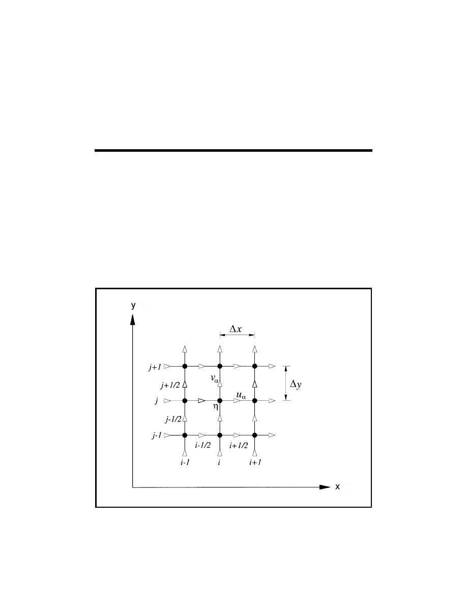
y directions, respectively. The equation variables η, uα, and vα are defined at the
grid points in a staggered manner as shown in Figure 3. The water depth and
surface elevation are defined at grid points (i,j), while the velocities are defined
half a grid point on either side of the elevation grid points. The external boun-
daries of the computational domain correspond to velocity grid points.
Figure 3.
Computational grid for finite difference scheme
12
Chapter 3 Numerical Solution

 Previous Page
