

1
Analysis
The wave record analysis utilized the Welch, [1], spectral analysis method with 50%
overlapping segments. Since the raw time series were obtained using sub-surface pres-
sure systems, a depth determined high frequency cutoff was applied. The averaged
co-and quad-spectra from each analyzed record were used to calculate significant wave
height (Hm0), peak period (Tp), and energy spectrums.
Hm0 Comparison
2
One way to evaluate the performance of the wave absorber, is to look for a reduction
in overall energy. Figures 2&3, show the incident and transferred wave heights, Hm0i
the transferred energy is less than the incident energy.
To provide a more direct comparison of incident and transferred energy, a transfer
coefficient (xfer) can be calculated by dividing the Hm0t by the corresponding incident
Hm0t
xf er =
(1)
Hm0i
Figures 2&3, second plots, are xfer values for the months of April and May 2003.
The Hm0t values were interpolated so that time could be synchronized. The transferred
rate varies from 0.40 to 0.80 for most wave records, however, there are a few times
with the overall rate above 1.0. For the most part, these high xfers occured during low
energy times.
An average energy transfer value was calculated using records from 4/11/03 to
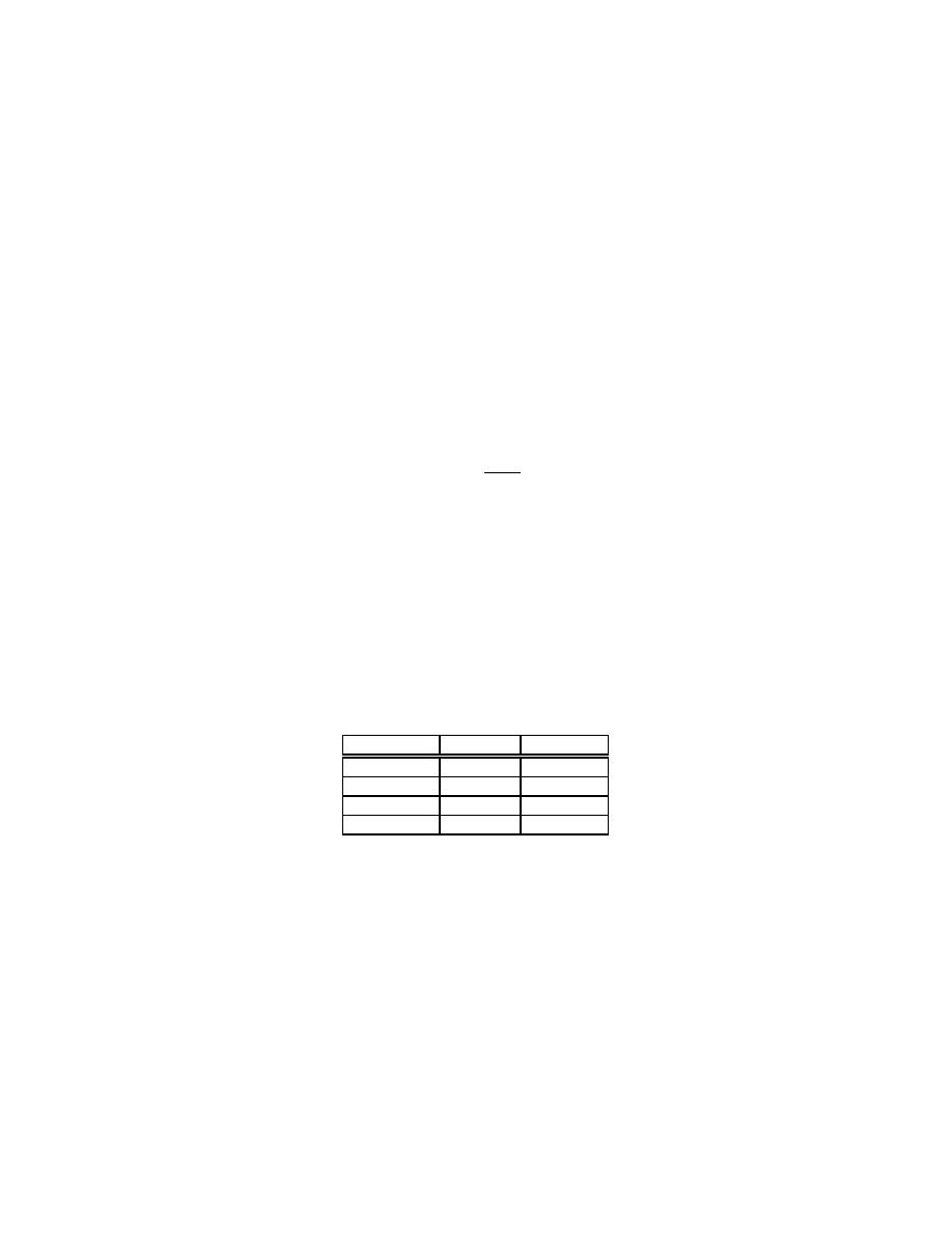
6/1/03 with various ranges of incident wave height. Table, 1, shows how the average
percent of incident energy transferred varies with wave height. The average transfer
rate using all 1206 available records and was 65.8%. Other averages were calculated
using only records with Hmoi > 0.1, >0.2, and >0.5 meters. The percent of energy
transferred increases with Hmo once we eliminate the very low energy records, Hmoi
<0.1 meters.
Hmoi
# Records
Transfer %
All records
1206
65.8%
>0.1 Meters
741
62.1%
>0.2 Meters
466
63.5%
>0.5 Meters
161
67.0%
Table 1: Average % energy transfer
fact 128 seconds. These very long period values were deleted from the plots for the
sake of clarity. Figure 4 contains 3 examples of pressure timeseries records. The time-
series plots contain 1024 seconds or 17 minutes of pressure data. The wave record is
dominated by a single wave of period about 17 minutes. Periodic water level move-
ment is evident in each plot.
3
Spectral Comparison
Figure 5, shows two spectral plots of successive wave records for both the incident and
the transferred gages. Note different time intervals. Most energy in both spectrums
2

 Previous Page
