

was decided that some exploration of the necessary number of directional components was
in order.
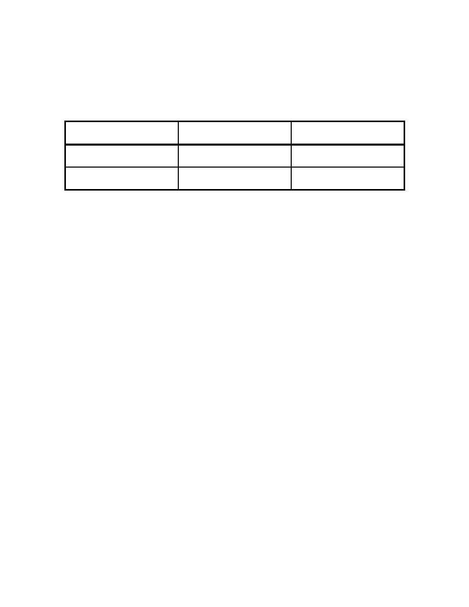
Table 3. Directional Resolutions Used for Model Input
∆θ (
)
Case ID
Number of Directional
Components (bins)
B1
9
20
29
4.14
N1
5
12
15
4
Tests were also performed to quantify the effects of the boundary conditions on
the solution. It was hypothesized that reflections from the coastal boundaries (simulated
walls of the wave tank) and improper treatment of these fully absorbing boundaries could
cause significant variations in the final solution, especially for components with large
angles of incidence. This hypothesis was tested by comparing the results obtained from
two domains. Domain A closely approximated the physical model and contained coastal
boundaries (Figure 11). Interior and exterior boundaries were considered fully absorbing
(KR= 0.0 and KEXT = 0.0). Domain B used a full circle as an open boundary and contained
all the depth variations (Figure 12). It was found that the boundary conditions do not
significantly effect the results from CGWAVE in the area of interest. Results are only
presented for Domain A.
CGWAVE results for the monochromatic conditions M1 and M2 are shown in
Figures 13 and 14. The wave amplitudes double behind the shoal and decrease on the
sides of the shoal.
The linear model results show a similar pattern. The non-linear
numerical calculations match the data better than the purely linear results. The data shows
that the maximum wave height occurs further behind the shoal than predicted by both
linear and non-linear solutions (section 7, Figures 13 and 14).
with ∆θ = 20
The CGWAVE results for the B1 spectral wave condition
discretization is shown in Figure 15. The result exhibits finger-like areas of large and
82

 Previous Page
