

conservation models with a depth-limited breaking criterion and simpler tech-
niques such as shoaling the component wave systems independently of each
other and superimposing the results. None of these techniques could reproduce
the observed changes to the wave spectrum.
Boussinesq model simulations were carried out for test case 7 in the Smith
and Vincent experiments. The sea state is composed of two irregular wave
components described by TMA spectra with Hmo,1 = 7.6 cm, Tp,1 = 2.5 s, Hmo,2 =
13.2 cm, Tp,1 = 1.75 s, and γ = 20. The numerical wave flume is 41 m long and
consists of a 20-m-long constant-depth region and a 1:30 planar beach. The water
depth in the constant depth section of the flume was 0.61 m. The measured time
series at the offshore gauge was used to generate velocity boundary conditions
for the numerical model. A grid spacing of 0.125 m and time-step size of 0.04 s
was used for the numerical simulations.
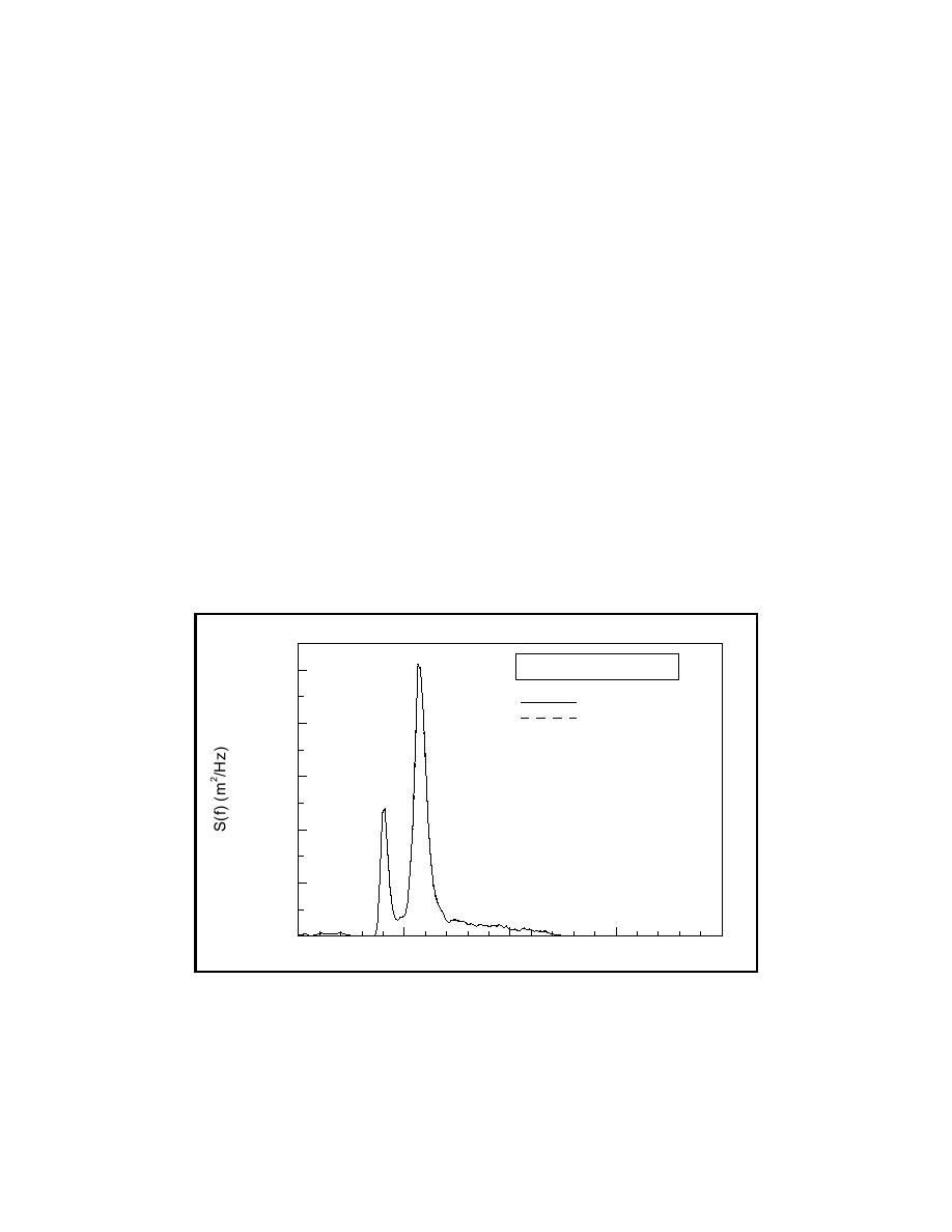
Figures 19 to 22 show comparisons of the measured and predicted wave
spectra at gauges located in water depths of 61 cm, 18.3 cm, 9.1 cm, and 6.1 cm.
Although the higher frequency component dominates the incident wave spectrum
with 67 percent of the wave energy at h = 61 cm, its energy is preferentially dis-
sipated with the lower frequency component becoming dominant at the shallow
depth of 6.1 cm. The Boussinesq model is able to reproduce the observed trends
in the experimental data. The primary reason for the preferential reduction in
energy of the high-frequency component is due to the nonlinear cross-spectral
transfer of energy during the shoaling process.
Water Depth = 61cm
0.01
Measured
Predicted
0.008
0.006
0.004
0.002
0
0
0.5
1
1.5
2
Frequency (Hz)
Figure 19. Measured and predicted wave spectra at Gauge 1 for bimodal sea
state shoaling on a constant slope beach
49
Chapter 5 Model Validation

 Previous Page
