

j
P
Γ
where { η } is the subset of { η } for
$
$
i
nodes situated on boundary Γ :
θP
Ω
{ } = {η , η , η
}
T
ηΓ
Γ
Γ
Γ
, ... , ηΓΓ
$
$ $ $
$N
1
2
3
1xNΓ
(55)
Γ
and
[K4]
is
a
fully
populated
N Γ M matrix :
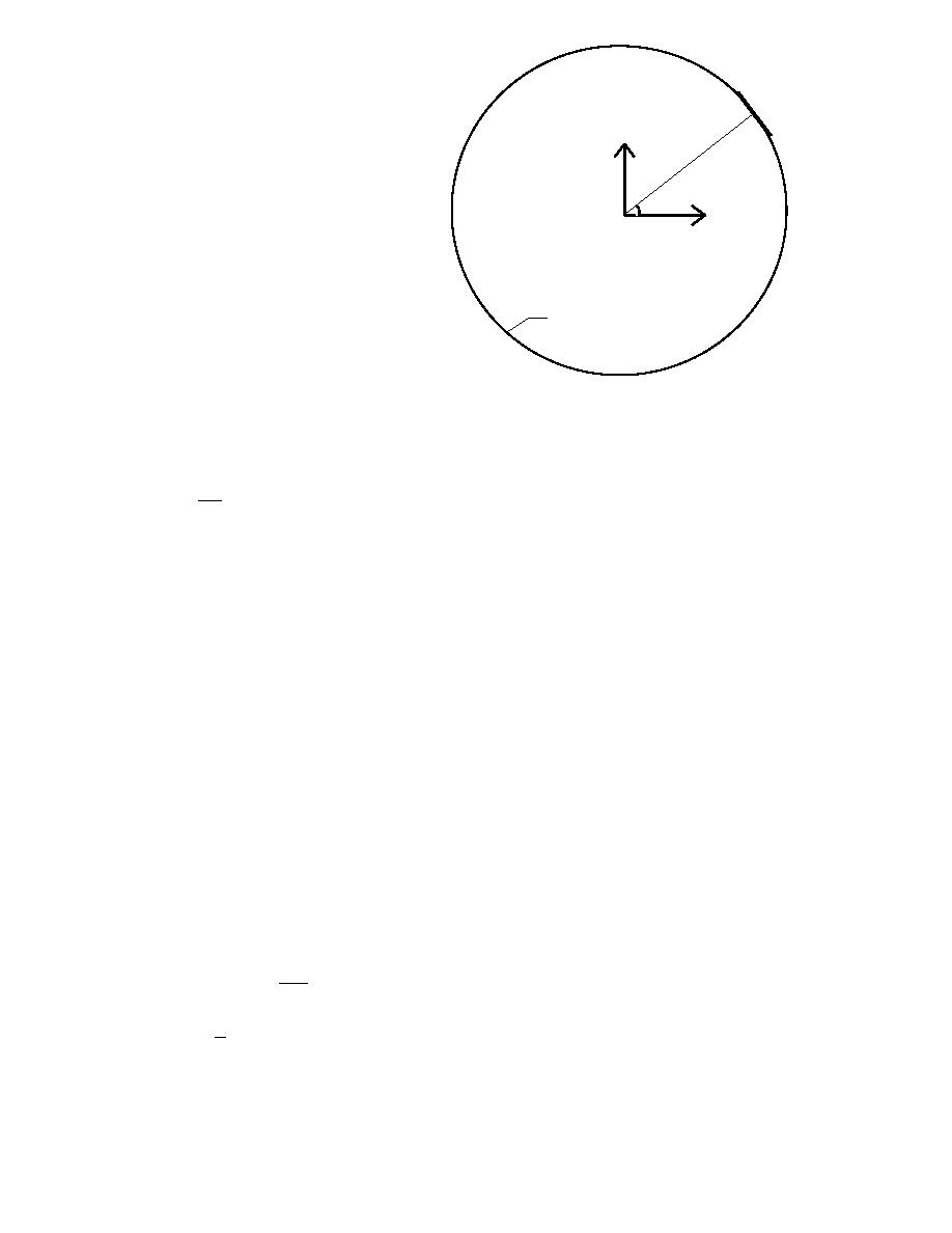
Figure 5. Definition sketch for line integrals
along the open boundary Γ
k~
a
[
K 4 ]=
2
(
)
(
)
H 'n sin nθN Γ- 1 + sin nθ1 L1 ⋅ ⋅
2H '0 L1 ⋅ ⋅ H 'n cos nθN - 1 + cos nθ1 L1
⋅
⋅
Γ
2H 0 L ⋅⋅ H n (cos nθ1 + cos nθ2 )L
H n (sin nθ1 + sin nθ2 )L
⋅⋅
⋅
⋅
' 2
'
2
'
2
⋅
⋅
⋅
⋅
⋅
⋅
⋅
⋅
⋅
⋅
⋅
⋅
⋅
⋅
⋅
' NΓ
(
)
(
)
2H 0 L ⋅⋅ H 'n cos nθN Γ - 1 + cos nθN Γ LN Γ H 'n sin nθNΓ - 1 + sin nθNΓ L2 ⋅ ⋅
⋅
⋅
(56)
where n = 1, 2, ..., m.
The next integral in Equation 45 is I5. Similar to the treatment in I4, we will take
the center value of η I/ n and assume linear variation of η for a segment on boundary Γ.
$
$
Substituting η I in I5 by Equation 15, it is easy to find
$
η
$
I5 = ⌠ ~η I ds
a$
⌡Γ
n
i ~ NΓ P P
(
)
[
]
= k a A ∑ L ηi + ηP cos(θP - θI )exp ikRcos(θP - θI )
(57)
$
$j
2
P=1
{}
= {Q 5} ηΓ
T
$
23

 Previous Page
